An introduction to (and puns on) Bayesian neural networks
Thomas Bayes’ tomb is located at the Bunhill fields next to the Old St Roundabout in London, less than a few hundred metres from our office building.
Disclaimer and Introduction - Getting our prior-ities straight
Much of this blog is a summary of a lecture by the late David MacKay, and section 41 and 44 of his textbook - Information Theory, Inference and Learning Algorithms, Cambridge University Press, 2003.
Similar to our post on kernel methods, this is a way for us at Papercup to vent about our favourite subfields in machine learning that are not written about as much or as widely understood as trendier topics. There are also many other introductions to Bayesian neural networks that focus on the benefits of Bayesian neural nets for uncertainty estimation, as well as this note in response to a much discussed tweet. In this post, we aim to make the argument for Bayesian neural networks from first principles, as well as showing simple examples (with accompanied code) of them working in action.
The data and examples below are adapted directly from the lecture material and the original Octave code on David MacKay’s website. We rewrote these examples to keep the material accessible and show simple examples of Bayesian neural networks working in action, though we don’t argue for their practicalities. We did so using JAX to be really cool.
Two notebooks were used to generate the figures for the Single-Layer Perceptron classifier and the Multi-Layer Perceptron regressor. They also contain examples of Bayesian neural network approaches - Laplace’s approximation and Variational Inference - on top of the Langevin sampling method described in this post.
Single-layer perceptron classification - Prior experience
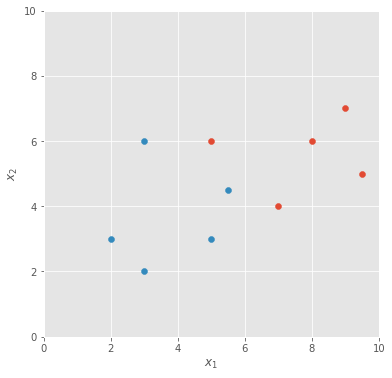
Suppose you want to classify some data points, such as the ones shown in the diagram below. Let be the location of the data points (and the inputs to our neural net), be the class of these points, and let’s use the letter to represent the entire dataset of points.
Let’s use a simple single-layer perceptron as our classifier, with three weights: , and for , and the bias, respectively, and a sigmoid activation function to obtain an estimate of the class probability. We make the assumption here that the neural net model we use is powerful enough to generate the dataset.
In maximum likelihood training, we adjust the weight parameters of our neural net classifier to maximise the likelihood of the data given the parameters, and we use it to make predictions on new data points. So let’s start by defining our loss function to be - the negative log-likelihood, which in this case is the binary cross entropy:
If we run batch gradient descent for some time, the classifier function settles into a state where the decision boundary is sharply in the middle between the two classes of data points.
Adding regularisation - Learning the Bayes-ics
Now, as David says in his lecture, you may well find the harshness of this classifier a little concerning, so we can introduce an additional penalty to our loss called “weight decay” or a “regulariser”, where we penalise the entire weight vector against having a large -norm. If we call this regularisation term , controlled by a hyper-parameter , it means our new loss function becomes:
With this new loss function, we’re able to train our model with more regularisation that is controlled by a hyper-parameter , where larger values of give us smoother decision boundaries after training.
Bayesian inference - The Silicon Valley Bayesian area
The Bayesian interpretation of what’s just happened here is that our regulariser is, in fact, enforcing a prior distribution - - over the weights, and that both the likelihood and the prior belong to the exponential family. The Bayesian approach focuses on the estimation of a posterior distribution - - over the weights, which can be calculated using Bayes’ rule:
is a constant, which doesn’t depend on the weight vector , and is therefore subsumed into the partition function .
This also means that what we’ve been doing previously has been finding the Maximum A-Posteriori (MAP) estimate , i.e. finding the weight vector that maximises the posterior probability. Note that when is zero (i.e. there’s no regularisation), we’re simply assuming a flat prior across the entire weight space.
Motivation - Marginalised by society
Why might you want to care about the whole distribution and not just the most probable weights?
David MacKay often uses an interesting example of a raffle game; consider a game where we have a very large bag of raffle tickets, let’s say infinitely large. On each ticket there is a sequence of 100 numbers, each number being 1 or 0, and each digit is i.i.d. Bernoulli distributed with probability of being a 1. The game costs £10 per go, and you get £1 for every 1 on the ticket you take out. Would you play this game? And if so what’s the amount of money you get? More formally:
We have two approaches: in the first approach, we concern ourselves with only the most probable ticket that we’ll pick out. The most probable sequence on a ticket would be one with all 0’s on it, with the exact probability being . We would refuse to play the game because if we pick out the most likely ticket, we’ll end up losing £10.
In a second approach, we may notice that is an incredibly small number (), and we may well work out that with 100 numbers on the ticket, the expected number of 1’s would be 20, so we’d expect to make a £10 profit from the game.
Presumably, most people would prefer the more intuitive second approach. Neural nets we use today have huge numbers of parameters and produce complex, non-linear functions, much less predictable than the simple reward function we have in the example; neural network weights are usually a float point, instead of a binary number, meaning a much larger weight space than the already intractable ticket space. If we want to use these functions to answer interesting questions, such as “which animals are on this image?”, we may well care about how these weights and functions are distributed.
Some “homework”: in what circumstances is the difference between the first and second approaches minimal?
The Bayesian interpretation - Bayes-ic instinct
Under the Bayesian interpretation, instead of viewing the weights of a neural net as variables to optimise, we now consider that there’s a whole distribution of weights that could have generated this dataset, and that there’s no longer such a thing as “neural net training”.
This perspective opens up some exciting questions: if there’s a whole distribution of weights, does it really make sense to only use one of them? What if we made our predictions taking into account all possible weight values?
Indeed! We can make predictions using Bayesian inference on any new data point by marginalising out weight vectors, therefore arriving at the marginal likelihood below. This is a powerful prediction as it is a prediction on the output dependent only on the input and the data .
Unsurprisingly, there’s some bad news, namely that the aforementioned partition function is generally intractable. Without them, we can’t really calculate the exact probability densities for any given weight vector.
Nonetheless, while we can’t work out the exact density function, we can still try to approximate it. These approximation methods largely fall into two approaches:
- Monte Carlo methods, which approximate the whole expectation through sampling using a distribution that converges to the posterior distribution, but not necessarily,
- And methods where we approximate the posterior distribution with another distribution, for example a multivariate Gaussian. Variational inference is one such method.
There are many great introductions on these topics, such as David MacKay’s lectures and textbook, or Kevin P. Murphy, Machine Learning: A Probabilistic Perspective, the MIT Press (2012).
We use Langevin Monte Carlo as an example of a Bayesian neural network approach, the notebook also contains implementations of Laplace’s method and a variational inference method.
Langevin Monte Carlo - MCMC Hammer
With a Monte Carlo method, we aim to draw credible samples from the posterior distribution, then estimating the marginal likelihood as the average of the outputs generated by the function using the sampled parameters.
The first example here is a Markov Chain Monte Carlo approach using Langevin sampling, where to get each sample, we simply perform batch gradient descent and add a bit of noise to it. The Langevin Monte Carlo method is also a special case of Hamiltonian Monte Carlo. An acceptance rule (Metropolis Hastings) is used to decide whether to accept or reject each proposed step we take, and we take samples once every few steps to reduce correlation between the drawn samples.
Below we show some of the sampled classifiers (produced by the sampled weights) we obtained from our Langevin Monte Carlo method - some of them similar to the trained classifier we had before, some of them less so.
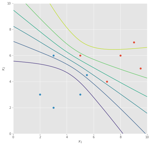
Averaging across all of these sampled functions, we obtain a marginal likelihood classifier that looks very different from before:
For starters, it’s no longer as “linear” as before, and while the classifier is just as certain in areas where we have data, it becomes less confident in its prediction as we move out to the upper-left and lower-right corner, i.e. regions where we have less data.
Uncertainties in the function space
Another question one might ask is: since each weight vector corresponds to a function represented by the output of the neural net, doesn’t that mean there’s a whole distribution of functions as well?
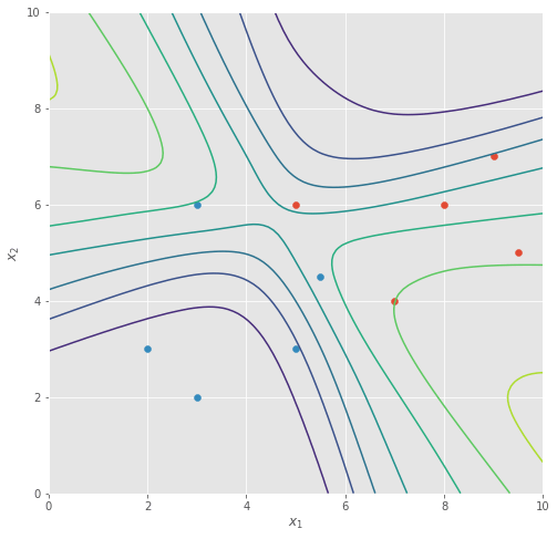
With a Bayesian approach we have uncertainty, or probabilities, over two spaces. We’re familiar with the probability distribution over the neural net weight parameters, which is the posterior distribution we’ve looked at so far. However since each weight vector produces a different function from the neural network, this distribution over the weights corresponds to a distribution over functions as well. The curved classifier above is essentially the mean function, meaning that we can also plot the function space standard deviation as well.
This plot of the standard deviation correlates with the confidence of the mean function plot.
Regression with a MLP - Variational on a theme
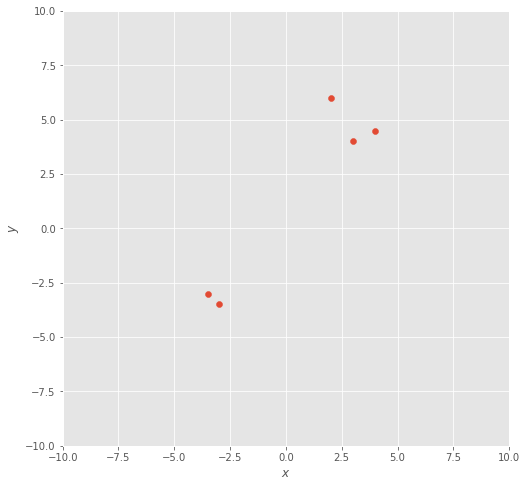
Let’s concern ourselves with another example of a regression task. Here both the input and output are one dimensional, with the objective being a curve-fitting exercise.
Let’s construct our neural net to be a multi-layer perceptron with a single hidden layer of 25 hidden dimensions with tanh activation functions and train our neural net with Mean Squared Error. Below is the progression of the model while training to maximise likelihood.
As our neural net is over-parameterised for the data we have, under maximum likelihood optimisation our model easily fits the data perfectly, producing a smooth function connecting all the individual data points together. Meanwhile, the MAP estimate produces a smooth, sigmoid-like function, assuming significant noise within the data.
More “homework”: are there cases in modern ML when we want functions to look more like the Maximum Likelihood answer? If we were reproducing real images pixel by pixel, does a Gaussian noise assumption, implied by the MSE loss, still make sense?
Nevertheless, let’s look at the Bayesian marginal likelihood again. Plotting out samples drawn from the Langevin Monte Carlo method, we obtain sampled functions which are slightly wrigglier than those from the optimisation approaches.
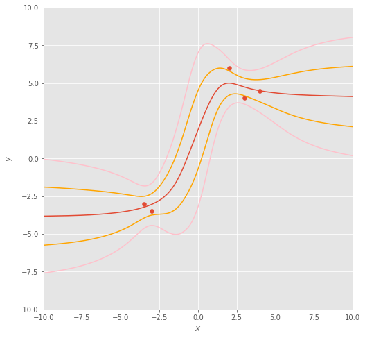
Should we plot out the mean function (in dark orange) along with 68% () and 95% confidence intervals () in orange and pink, respectively, we obtain a function distribution that’s more confident around locations where we have data, and less certain when we’re extrapolating ( and ) and interpolating ().
You may well say: “Great! This gives me a lot of information about my predictions!”
Even more “homework”: does this plot remind you of other Bayesian models? What if we could make Bayesian predictions by simply modeling the covariance of the output values between each of the data points instead, using a kernel method?
A side note and more puns - Latent to the party
Throughout this post, we’ve not really dived into a key assumption we’ve made, which is that the neural network model we use is the correct model used to generate the data in the first place, or that the model is powerful enough to generate the data. In more concrete terms, we’ve approximated the true marginal likelihood with one that is also dependent on the model choice :
Where represents everything about your model choice: the size, number and form of the layers, the choice of the activation functions, or even the question whether the model should be a neural network at all. It also means that all of the quantities we’ve seen are in fact also conditional on as well. We may want to pay attention to the fact that becomes , because we can then invent a model prior and concern ourselves with the quantity .
Thanks to Tian and Devang for their comments and suggestions!
The puns that didn’t make the cut
- Bayes-less accusations
- Bring the Gaussian noise
- My cherie amortised
- Better latent than never
- I think therefore EM
- Gibb or take
- Markov the things you’ve done
- KL’ing me softly
- GP KLinic
- Kernel Sanders
- It’s hip to be squared exponential kernel
Subscribe to the blog
Receive all the latest posts right into your inbox
