Subscale WaveRNN

You have read Efficient Neural Audio Synthesis aka the WaveRNN paper and would like to know more about how the subscale system works and how it can be implemented?

This blog post might appease your eagerness.

You’d also like a working PyTorch implementation to play around with?

Our accompanying repo subscale-wavernn might be right up your alley.

We found this idea very interesting and a fun engineering problem to solve, with a lot of room for imagination left for those willing to re-implement the system. So we gave it a go and are now ready to share our interpretation and code.

We will go though:

• Motivation behind subscale
• The high-level idea
• How subscale inference works
• Where it fits in the WaveRNN architecture
• Details about our implementation

Please do reach out for any comments / questions / requests - enjoy!

Autoregressiveness works wonders but… inference is slow

Autoregressiveness is a really sensible assumption when modelling audio - it very much reflects the physical nature of how speech is produced. Have a look here for an hands-on overview of basic autoregressive models. This article explains how human speech is a pressure wave (like any other sound) which originates in our lungs and vocal folds and is modulated by the topology of our vocal tract up to our lips movements. Let’s take the lips as an example of speech organ: intuitevely, the shape of our lips at time t is always dependendent on the shape at time t-dt. You can only modify the lips shape by x in a timespan dt; so knowing the shape at t-dt is incredibly useful information that you can regress against. Similarly for all other speech organs, which are responsible to create human speech. This is an oversimplified explanation, but it provides a barebone intuition as to why speech is often modelled using the autoregressive assumption.

Needless to say, this assumption translates into state of the art results in TTS output quality: see the tacotron 2 and wavenet papers for examples of how the autoregressive assumption is key to modellinig speech.

However, autoregressive models are fundamentally slow when it comes to inference time, especially when dealing with high clock rates like in waveforms. For high quality speech, we want 24khz and often we’d want more than just 1 second, so as you can imagine a hell of a long output sequence!

We can only generate sample by sample because each prediction is conditioned on the previous one and each step needs to wait until the previous one is completed. This seems incompatible with what GPUs and other hardware are good at: parallelization.

The itch is: we’ve got all this extra memory in the GPU free to exploit… we can’t just chunk up the input across the time dimension and batch the chunks together: we’d end up with glitches when stitching the output chunks back together. What can we do to exploit the batch dimension without decreasing output quality?

Can we trade some past for some future?

The idea behind subscale is to trade off past context for some samples in exchange of future context for other samples. For a target batch size $B$, this is achieved by having your RNN sampling at a $1/B^{th}$ of the waveform sample rate clockrate, with a time offset between each RNN. Each RNN of the batch sees a different amount of context based on what has already been generated. This way, at a given point midway through generating your waveform, you’ll be able to generate $B$ samples at the time.

Ok we get the high level idea… but how is it done in practice?

Getting this to happen in practice does require some clever engineering. Disclaimer: there are probably other ways to interpret what is described in the subscale part of the paper other than the few that we present here.

Let’s first introduce some concepts so that we can abstract them away in the later explanations:

1. Permutation

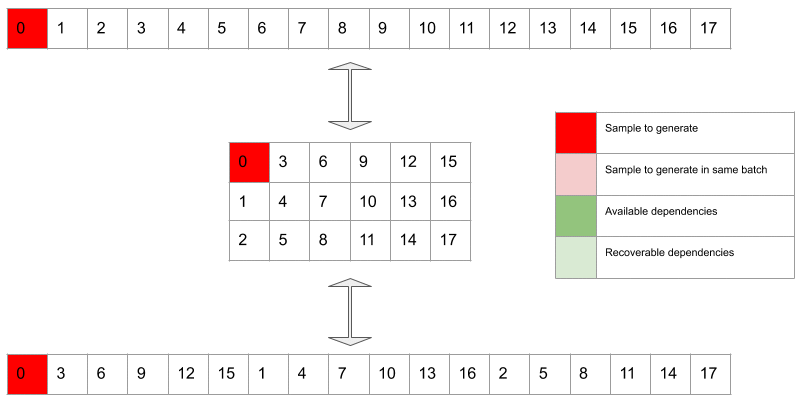
   We organize the target waveform in $B$ subtensors by grouping every $B^{th}$ element together. This is a permutation because we’re only manipulating the order of the samples. In the image, each color codes the membership of the sample to one of the $B$ subtensors (in all our examples we have $B=3$). In subscale inference, we can generate the $B$ subtensors in parallel (with an offset), and within each subtensor we’ll generate by following the permuted order.

2. Future horizon

   The future horizon $F$ represents the number of $B$-sized groups of future samples that are in principle eligible to be seen by the network as context when generating a sample. $FB - 1$ is the offset between samples that can be generated in parallel, in the same batch. In our examples $F=1$, and in the picture below the target sample is sample number 7.

How is the batch constructed?

This is best appreciated visually, so you are welcome to jump to the gif below and read this after. I’d also recommend unpacking the gif and go through each frame in your own time. A more wordy explanation in this paragraph.

Given the hyperparameters $B$ and $F$ and a target waverform at clockrate $sr$, we permute the target waveform into $B$ subtensors which run at clockrate $sr/B$ per second, each containing samples from the original waveform at $B$ distance between each other.

When generating a sample $T$, belonging to the $N^{th}$ subtensor, the network has access to all the previous samples belonging to $N^{th}$ subtensor:

N, N + B, N + 2B, N + 3B, N + 4B...
etc. up to T - B

as well as all samples from $0$ to $T + FB$ belonging to the $0^{th}$ to $(N-1)^{th}$ subtensors:

0, 1, 2... N,    B, B + 1, B + 2... B + N,    2B, 2B + 1, 2B + 3... 2B + N,   ...
etc. up to T + FB.

Let’s go trough it step by step for $B=3$ and $F=1$:

• First, we generate sample $0$ which belongs to the $0^{th}$ subtensor. At this stage, the batch size is $1$ as we’re only filling up one subtensor.
• Now we can generate the next sample in the $0^{th}$ subtensor, i.e. sample $3$. Batch size is still $1$.
• Sample $0$ and $3$ are available, so we can generate sample $1$, which is the $0^{th}$ element of the $1^{st}$ subtensor, as well as sample $6$ to continue filling up the $0^{th}$ subtensor. Batch size is now $2$, as we’re filling up both the $0^{th}$ and $1^{st}$ subtensors.
• The samples available are now $0$, $1$, $3$ and $6$. It’s still too early to start generating the next and last subtensor, as we’re missing sample $4$ which is required to generate sample $2$. However, we can generate $4$ and $9$ together (batch size of $2$).
• Now we’ve got everything to exploit the full batch size of $3$ as we can generate $2$, $7$ and $12$ together. Sample $2$ requires $0$, $1$, $3$ and $4$, sample $7$ requires $0$, $1$, $3$, $4$, $6$ and $9$ and sample $12$ only needs $0$, $3$, and $9$.
• And similarly for the remaining steps. The same principle still holds at the end. This time, with the $0^{th}$ subtensor finishing first, the $1^{st}$ second, and so forth. This means that some of the future context become unavailable for the higher-order subtensors, as they are out of range. E.g. if the waveform is only $18$ samples long (so the that the last one is sample $17$), when generating sample $16$ we’re not goinig to have sample $18$ and when generating sample $17$ we won’t have $18$ and $19$.

You might have noticed that there’s quite a difference between the $0^{th}$ subtensor and the other ones. The $0^{th}$ subtensor is generated completely independetely from the other $B - 1$ subtensors, and it behaves more like the classic autoregressive manner where each sample is conditioned on the previously generated ones, with no extra clues from future samples. The other subtensors instead seem to have an easier task, since if you already know what sample is next and what sample was before, if you interpolate the two you probably already get a good guess. In our experiments, this is reflected in the loss: the loss can be broken down into $B$ losses, one specific to each tensors. And the loss relative to the $0^{th}$ subtensor is always higher than the successive ones.

Gif 1. In dark green are the available dependencies, i.e. samples used to condition the network when generating a target sample (in dark red). The light green samples are recoverable dependencies relative to the dark red sample. These are samples that could in principle be accessed when generating the dark red sample because they have already been generated at previous steps. However these are deliberately discarded by design choice. Light red samples are target samples that can be generated in the same batch in which the dark red sample is generated. Please note that samples corresponding to recoverable dependencies relatively to the dark red sample can be available dependencies for the light red target samples.

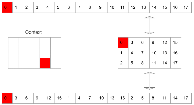
How is the context information fed to the network?

The paper is not explicit about this so we can’t guarantee this is exactly what the authors meant, but rather what seems most plausible to us given the information available.

A basic autoregressive RNN cell takes an input features frame $I_{t}$ (in our case the upsampled MFBs, mel filter bank feautres) as well as the output from the previous step $O_{t-1}$ and generates $O_t$. Training happens in teacher forcing mode, i.e. by feeding the ground truth $O_{t-1}$ as the RNN inputs.

In subscale WaveRNN, we don’t just condition on $O_{t-1}$, but rather on a wider window of outputs (ground truths during training and generated during inference), whose range depends on the subscale parameters (batch factor, future horizon and context width). Let’s call this window of outputs the context.

The context is fed thorugh a conditioning network whose output replaces the traditional $O_{t-1}$ in the RNN cell input.

Img 1. The conditioning network condenses the information contained in the context, which is extracted from the waveform, and is equivalent to the previous output sample in the standard, non-subscale settings.

How is the context constructed?

To get the context, we need to select the right window of samples from the waveform. At training time, we use the ground truth waveform and all samples are available, so we only need to mask the window of samples in a way that simulates which samples would be actually available at inference time.

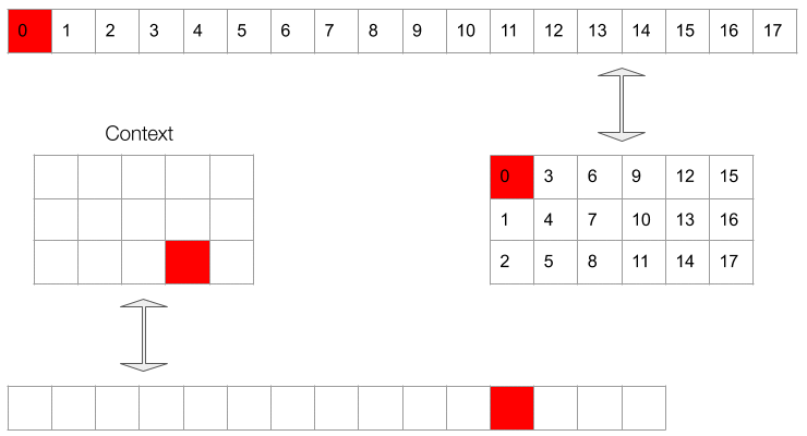
The main intuition when trying to implement this was that at any step $t$, the RNN has no notion of how far into the MFB squence it is reading, and therefore, the way the context is constructed needs to obey the same invariance. By design, the right-hand side boundary of the context window is in the future relative to the target sample. So the $(FB + 1)^{th}$ entry from the right will always be empty as it represents the target sample.

The left-hand side boundary of the context needs to be fixed but it’s arbitrary. It basically reflects how far into the past you’re looking back to.

The context is masked based on the subtensor’s membership of the target sample. This can be seen when permuting the window similarly to how the target waveform is permuted when running the subscale inference. For example when the target sample belongs to the $0^{th}$ subtensor, all entries in the context corresponding to samples belonging to the $1^{st}$ to the $B^{th}$ subtensor will be blank, as well as the samples belonging to the $0^{th}$ subtensor that are in the future relative to the target sample. For the other subtensor, the masking follows from the same principle as in the first section of the blog post, and is best illustrated in Gif 2.

Gif 2. The context is a masked window of the waveform which is fed to the conditioing network. The masking at training time needs to simulate the available dependencies at inference time.

Another way of visually constructing this is overalying a context-shaped tensor (left rectangle in Gif 2) over the permuted waveform (right rectangle in Gif 2). Use the target sample position - which is always the same in the context - to set the matched location. Then you can visually slide the context shape over the waveform to find out which samples are available dependencies and which positions they should be locate at into the context.

The reason why the target sample needs to always be in a fixed position in the context is because of the above metioned invariance: the network needs to learn the relationship between the target sample and the available dependencies in the context in a way that is generalizable across the whole sequence. In other words, the relative distance in the context between $t$ and $t \pm t_0$ must be the same for all $t$.

It’s easiest to picture the masking in the 2d permuted representation. However, what the conditioning network sees is actually a 1d vector which follows the same ordering as the original waveform. This can be appreciated in Gif 3.

Gif 3. The context (bottom sequence) as seen by the upsampling network.

It will be up to the conditioning network to condense the context information in a way that the RNN can make the best use of it. Ideally, when the context is rich and many future samples are avaialable, the RNN should maximally exploit that, to the extent that the MFBs almost become insignificant. Whilst when the context is poor, the RNN should rely heavily on the MFBs and the most recent available output samples.

The job of the RNN cell is vastly different for each of the subtensors, to the point that one wonders whether in the original implementation they actually had a different set of rnn weights for each subtensor, effectively leveraging $B$ RNNs. In principle, these could be stacked together into a single layer run or simply run in parallel. However this would mean increasing the total number of (RNN) weights by $B$ times. At that point if you have 1 RNN per subtensor then why not 1 conditioning network per subtensor as well?

This leads us to guess that it is the same RNN and conditioning network that learns all these different tasks, just by virtue of learning the different “modes” of the conditioninng network’s output (which reflect the $B$ modes of the the context). And it’s actually the training routine that can be engineered to encourage the model to learn the desired behaviour.

How is it trained?

This is more of an open question for us, as we haven’t experimented much with it. For now we will limit ourselves to write some considerations to spark the discussion. We also encourage everyone to use our implementation to experiment with different trainining routines and subscale hyperparameters.

At training time, we can compute the loss for all the different subtensors and confirm that gerating samples from the $0^{th}$ subtensor is indeed the hardest (and loss is highest).

A spontaneous worry arises: at inference time, each subtensor relies on outputs from the previous subtensors, so if the $0^{th}$ subtensor is hard to generate, the error will compund when generating samples in the following subtensors. Because at training time we use samples from the ground truth waveforms, the typical discrepancy between inference and training time performance could be amplified.

One way to engineer the training routine could be to weight the partial losses differently. Or possibly learn the weighting dynamically using Lagrange multipliers.

Since at training time, the masking is done artificially, we could set up a “curriculum”, where we first show the network the easy cases (more context) and gradually increase the percentage of lower context samples. Or vice versa!