Ctrl-P: Temporal Control of Prosodic Variation for Speech Synthesis
Things have been a little quiet on the blog in the last year, but we’re back and excited to share that Papercup will be presenting two papers at Interspeech 2021! You can check out ADEPT which introduces a dataset for evaluating prosody transfer in another post. This post will cover the Ctrl-P model. We invite you to also listen to the accompanying audio samples on our samples page.
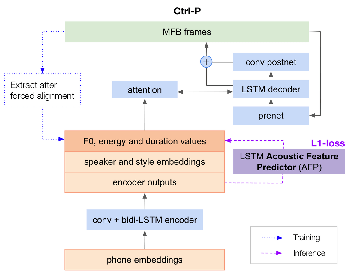
One of the fundamental challenges of TTS is that text does not fully specify speech; the same text can be said in many different ways. Ctrl-P approaches this one-to-many mapping problem by using acoustic information as an additional learning signal, thereby reducing the unexplained variation in the TTS training data. We explicitly condition the model on the three primary acoustic correlates of prosody - F0, energy and duration - at the phone level. During inference, these acoustic feature values are predicted from text, with the option to subsequently be modified by an external system or human-in-the-loop to control the prosody of the generated speech.
Controllability requires a system to respond predictably and reliably to its levers of control. We show that Ctrl-P provides more interpretable, temporally-precise, and disentangled control compared to a model that learns to extract unsupervised latent features from the audio. By ‘temporally-precise’ we mean both the ability to perform control at specified locations and for those changes to result in localised changes in the generated speech.
We also demonstrate Ctrl-P to be more reproducible and less sensitive to hyperparameters, which is crucial for any deployed system. This was actually one of the main initial motivations that led us to this approach.
How does this work differ from related works?
Many recent works in TTS have tackled expressive speech synthesis and prosody modelling. We note two main points of differentiation from prior work. First, we model the acoustic variation explicitly with extracted acoustic features. This is distinct from the body of work that models acoustic variation implicitly as a residual component captured through a latent space, commonly in the form of an embedding of the reference mel spectrogram (Wang et al. 2018, Skerry-Ryan et al. 2018, Sun et al. 2020).
Second, our work provides precise and localised control over all of F0, energy and duration at an appropriate temporal granularity that balances the competing requirements of i) accounting for unexplained acoustic variation, and ii) providing intuitive control for a human-in-the-loop. Other works that have similarly used extracted acoustic features as additional TTS input have either had a more limited set of features (Łańcucki 2021), modelled the features at a level that only allows coarse control at the utterance level (Raitio et al. 2020), or modelled the features at a temporal resolution that is too fine-grained for human control, e.g. at the frame level (Ren et al. 2020, Lee et.al 2019).
That said, both the idea and the model we arrived at are quite simple and not technically too different from recent related work. Perhaps the main value of our contribution is in our focus on the controllability aspect of the model, as we serve a product that integrally involves human-in-the-loop. We were especially keen on the notion of separating prosody modelling from the generation of speech by the core TTS model as it allows us to build control features and transfer prosody by interacting only with the prosody network, and opens up the avenue of training the prosody network on non-TTS grade data.
Nuts and bolts (rather, layers and losses)
Ctrl-P is built on top of a multi-speaker (and multi-style) variant of Tacotron 2 (Shen et al. 2018). We modified Tacotron 2 in the usual way, simply concatenating speaker and style embeddings to the encoded phone sequence, or encoder outputs, which the decoder subsequently attends over when generating speech.
For Ctrl-P, the only addition we make is to explicitly compute three acoustic feature values - one each for F0, energy and duration - for each phone. We compute F0 and energy values from the waveform and average per-phone after forced alignment using an aligner trained on our TTS training data. Duration is represented as the number of frames. Acoustic features are z-normalised on a per-speaker basis across the entire training set, then concatenated to the encoder outputs. We also experimented with log feature values and per-utterance normalisation, but both degraded performance.
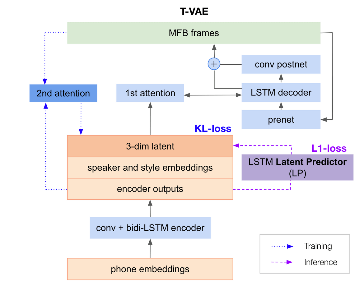
We compared this against a temporal variational auto-encoder (T-VAE) that learns a 3-dimensional latent feature vector for each phone. This model has a secondary attention mechanism that aligns the reference mel-spectrogram to the phone sequence during training to produce a corresponding sequence of 3-dimensional latent vectors. An additional KL divergence loss term is applied to the latent space.
At inference time, both the acoustic feature values in Ctrl-P and latent values in T-VAE are predicted from the encoder outputs with a (acoustic feature / latent) predictor network (AFP / LP). The predictor network architecture is identical for both models, consisting of two bi-directional LSTM blocks that are trained on the L1 loss against the reference acoustic feature values, and the latents produced from the reference mel spectrogram, respectively.
The models were trained on a proprietary, multispeaker, Mexican-Spanish corpus consisting of approximately 38 hours of speech in multiple styles. We followed a two-stage training routine. First, we train everything except the AFP / LP for 200k iterations. Reference acoustic feature / latent values are used at this stage. Then, the AFP / LP is trained for 400k iterations with the rest of the model frozen. We experimented with letting the encoder weights also train during the second training stage, just to see if the AFP might improve, but found no perceptible difference. In principle, the AFP and LP could be concurrently trained with the rest of the model, but we kept the two-stage routine in order to easily and quickly experiment with different predictor network architectures.
For the subjective naturalness evaluations, we vocoded the samples with model-specific WaveRNNs trained on respective model-generated mel-spectrograms. For the objective controllability evaluations, the large number of waveform samples required were vocoded with Griffin-Lim.
Ctrl-P offers several advantages over T-VAE
1. Disentangled control
To inspect the disentanglement of control over each acoustic feature, we modified the entire contour of each input feature and latent dimension by shifting it a fraction of the per-speaker standard deviation for that dimension, leaving the other two dimensions unchanged. The average change in utterance-level F0, energy and duration of the synthesised output was then measured.
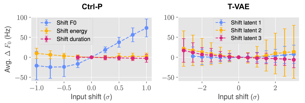 Objective evaluation of disentangled control. x-axis: fraction of the speaker-specific standard deviation by which the feature (or latent) was shifted. y-axis: average resulting F0 change in the output. Points represent the mean; whiskers denote one standard deviation. Similar results were observed for energy and duration.
In Ctrl-P, only shifts in F0 input value (blue line) result in changes in average F0 of the synthesised output. Shifting energy and duration (yellow and pink lines) leaves the output F0 relatively unchanged. In contrast, all latent dimensions affect output F0 in T-VAE. In fact, every latent affects more than one acoustic feature in the output (see paper for more plots), thus we say that T-VAE produces entangled changes. Observe that with T-VAE, the direction and magnitude of change can be inconsistent across utterances, as seen from the wide standard deviation bands, most noticeably in latent 2 (yellow line).
2. Temporally-precise control
To assess the temporal precision of control, we randomly selected a subset of the stressed vowels within an utterance and shifted each feature (or latent) dimension in turn for that phone, leaving other phones unchanged. Forced alignment was then performed on the output waveform and F0, energy and duration changes were measured for each phone.
 Objective evaluation for precision of temporal control. Results are averaged across all validation set utterances for a randomly chosen female speaker. Similar behaviour was observed for all speakers. See the paper for similar results for energy and duration.
Ctrl-P achieves temporally-precise and disentangled control of only the intended phones (pink bar), with other phones remaining relatively unchanged (blue bar). In contrast, the temporal region of influence is unclear for T-VAE, with both the modified and unmodified phones undergoing changes in acoustic properties.
3. Model reproducibility
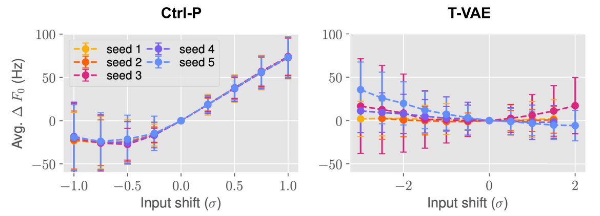
We trained Ctrl-P and T-VAE from different random seeds, and repeated the same analysis for disentangled control on the different models to objectively assess model reproducibility.
Objective evaluation of model reproducibility. Shifting the input F0 value in Ctrl-P resulted in consistent and predictable F0 changes in the output speech across random seeds. Conversely, shifting the latent values in T-VAE (for this plot, we arbitrarily chose the 1st latent-dimension) resulted in unpredictable F0 changes across random seeds. Similar results were observed for energy and duration - see the paper for complete results.
The effect of shifting the T-VAE latent dimensions varies substantially across random seeds. We did not observe the same sensitivity in Ctrl-P, which was what we expected given the explicit supervision.
Subjective Evaluation of Naturalness
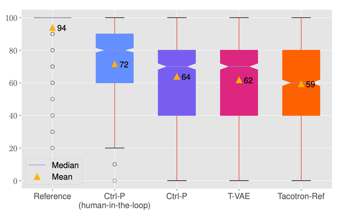
We conducted a MUSHRA-like (the scale was modified to have intervals of 10) subjective listening test of a randomly chosen selection of 5 validation utterances each from 6 speakers (3 male and 3 female). 50 self-reported Spanish-speaking listeners were recruited via Amazon MTurk. As a benchmark for naturalness, we included the well-established Tacotron 2 with reference encoder (Tacotron-Ref). We also included human-in-the-loop controlled samples for the Ctrl-P model, where the acoustic features predicted by the AFP were modified by a human, aiming for higher fidelity to the original reference.
Results from a MUSHRA-like subjective evaluation of naturalness. Each box spans the 1st to 3rd quartiles (Q1, Q3); whiskers denote the range (capped at 1.5×(Q3−Q1)); outliers are shown as individual points.
All model pairs statistically significantly differ in naturalness. These results suggest that Ctrl-P is able to produce more natural speech than T-VAE (though only marginally) and Tacotron-Ref. More importantly, human-in-the-loop control of the Ctrl-P acoustic features was able to achieve a substantial further increase in naturalness.
The temporal precision offered by the model enabled our quality assurance annotators to make targeted adjustments to the rhythm, intonation and word emphasis within an utterance, enabling prosodically distinct renditions of the same text.
Further work
Going forward, we would like to expand the feature set to include other acoustic correlates of prosody, such as spectral tilt or segmental reduction, and improve the AFP to obtain better ‘default’ prosody. We are also interested to explore ways in which the model can generalise beyond the range of feature values in the training data, as we observed diminishing effects of control towards the extremes of the region of seen values. Finally, we are eager to explore ways to build more abstract and efficient levers of control atop Ctrl-P, such as ‘emphasise this word’, or ‘create rising question intonation’.
B-roll
Papers tend to present the research process as a linear one. This is necessary for clarity and conciseness, but is often far from what happens in reality. Like many other researchers, we too ventured into many deadends, made u-turns and encountered oddities. Many of these were not included in the paper, but we think they can be just as valuable to share.
We wondered why the plots for disentangled control curved towards the ends. As mentioned, anecdotally, the main reason appears to be the model’s limited ability to generalise to feature values beyond what is seen during training. It is worth mentioning that we observed variation across speakers - some speakers had a straight-line response within the range of shifts that we applied. We also wondered why the response was not symmetric. This is likely a statistical effect - we computed the z-normalisation statistics in a naive way over all phones in the utterance, not distinguishing between voiced and unvoiced phones, as well as silences. As such, the computed mean may not always be equidistant from both ends of the range of seen feature values.
We observed that the acoustic feature values sometimes served as proxy for mistakes in the recording, noise and artifacts in the data and phonemisation errors. For instance, a silence token with a high energy value could indicate noise or speaker hesitation and Ctrl-P seemed to probabilistically generate them in the output accordingly. In fact, for certain speaker-style combinations, we actually observed that increasing the input energy values resulted in louder background noise rather than an increase in speaking volume.
We also looked into whether the input-output control response was 1-1 in the raw feature value, i.e. if we shift the input by an equivalent of 10 Hz, do we observe the same 10 Hz change in the output. We assessed this in the same way as Raitio et al. 2020, and found that only duration had a close to 1-1 response. F0 had a weaker than 1-1 response (slope < 45˚) while energy had a stronger than 1-1 response (slope > 45˚). Note that an equivalent analysis could not be done for T-VAE.
As some of you might have guessed, we actually started developing the T-VAE model first and switched to the Ctrl-P model later as we struggled with model reproducibility and training stability. We showed in the paper that different random seeds can lead to very different latent spaces in T-VAE, but the inconsistency was exacerbated when we trained on different multilingual data combinations, where we had to carefully tune the weight on the KL divergence loss and fiddle with the training routine to avoid posterior collapse. Sometimes, the second attention would not learn at all.
When we initially made the switch from T-VAE to Ctrl-P, we couldn’t get the AFP to predict natural-sounding prosody. In response, we tried a more complex, linguistically motivated hierarchical architecture and were rather pleased with ourselves when it finally worked. However, in the process, we had inadvertently made the AFP larger as the hierarchical model had more layers. It wasn’t until we did an ablation that we discovered that the initial simpler architecture worked just as well, once we controlled for the number of layers and model size. Abiding by Occam’s razor, this simpler model was the one that became Ctrl-P. While it was initially a little meh to learn that the thing we took pride in building wasn’t quite as cool as we thought, it was for the better, and we were reminded that sometimes it’s best just to stay simple.
That’s it! Thanks for sticking around until the end and taking an interest in our research 🙂 We’d love to hear your thoughts, questions and comments on any of our work, so feel free to drop us an email. ‘Til the next time!
Subscribe to the blog
Receive all the latest posts right into your inbox
