Tutorial on normalizing flows, part 1

Before we start, I would like to mention that this blog post assumes a familiarity with generative models and modern deep learning techniques.
Furthermore, if you would like to jump ahead to the tutorial, please visit our tutorials page: https://github.com/papercup-open-source/tutorials.

Generative models are a very popular topic in the machine learning literature. From Generative Adversarial Networks (GANs) to Variational Auto Encoders (VAEs), it is undeniable that a very big chunk of the papers being published at the top ML conferences (NeurIPS, ICLR, ICML) seem to have some form of generative modelling incorporated into it. They are fascinating, as they can allow us to get a better understanding of the underlying structure existing in our datasets (eg the latent space of a VAE trained on MNIST might cluster per digit). For example, they have permitted, through GANs, generation of extremely high fidelity images which are capable of fooling human beings into believing that they are photos of real people. The list of uses goes on and on.

One particularly interesting subclass of generative models is called flows. They have become popular recently, and have received quite a lot of attention — for example Glow, by OpenAI — because of their immense power to model probability distributions. Flows have been widely used in speech processing, most notably through WaveGlow (NVIDIA), but also more recently by Amazon in this paper. I will not go in depth in explaining what a flow is, since others have done it very well, and I do not pretend to have a better understanding of it than they might. If you are interested in the maths of it, I recommend reading this article, as it is very well explained.

In theory

What I will do, however, is run you through an example of how normalising flows can be used to approximate a very complex probability distribution.

We want to learn an “in-the-wild” distribution implicitly. Note that here, this refers to an arbitrarily complex distribution. Let us assume that we have data sampled from one such “in-the-wild” distribution. For example, this could be handwritten digits (MNIST) or house prices as a function of square footage. We would like to approximate this distribution through generative modeling. In practice, what we will do is to first define a sequence of invertible transformations $f_1, f_2, ..., f_T$ with upper (or lower) diagonal Jacobian matrices. The motivation for this is the same as stacking multiple linear layers with non-linearities in between in regular neural networks - it allows to model more varied distributions.

Let $Z_0 \sim N(0, I)$. We define random variables

$Z_i = f_i(Z_{i-1}), \ \forall i = 1, \dots, T$

Then, I claim the following - given the probability distribution of $Z_0$, and the parametrisation of $f_i$, for all $i$, we can obtain the probability distribution of $Z_T$. Moreover, since the $f_i$’s are invertible, given samples $\{x_j\}_{j=1}^{N}$ from an “in-the-wild” distribution $X$, we can parametrise it as

$X = Z_T, Z_T \text{ defined as above}$

where the $f_i$’s are modelled as invertible neural networks, and optimise these weights according to the data $\{x_j\}_{j=1}^{N}$ with maximum likelihood. Easy enough, right? We will give an example of such a distribution in the “In Practice” section.

For more details regarding the math of this claim, please refer to the blog post linked above. If you are interested, I would refer you to the “Change of Variables in Probability Distributions” section in the linked post. The only thing that you need to retain here is that we know the exact probability distribution of $Z_T$, because the $f_i$’s are invertible. This allows us to perform maximum likelihood estimation on the weights parametrizing the $f_i$‘s. I will however leave you with the formula for the likelihood of $X$ according to the above model:

$\text{log}(p(X)) = \text{log}(p_{Z_T}(Z_T)) = \text{log}(p_{Z_0}(Z_0)) - \sum_{i=1}^K \text{log} \left| \text{det} \frac{\text{d}f_i}{\text{d}Z_{i-1}} \right|$

This shows why knowing the probability distribution of $Z_0$ (which we do, since we defined it as $N(0, I)$), and the determinant of the jacobians $\frac{\text{d}f_i}{\text{d}Z_{i-1}}$ (which we do, by design of the transformations $f_i$), then we can figure out the exact likelihood of $X$, and can optimise for it. Note that the functions that we have defined are neural networks, and as such are parametrized by weights which we need to optimise in order to find the optimal functions given the “in-the-wild” data.

Even cooler is that once the network is trained, we will have access to a sequence of transformations which allow us to sample from $N(0, I)$, and through sequential application of the transformations, approximate a sample from any “in-the-wild” distribution. Let us see how we can actually use this in practice.

In practice

This section of the post borrows heavily from a tutorial run by Eric Jang at ICML 2019.

We have adapted it to PyTorch with additional bits here: https://github.com/papercup-open-source/tutorials.

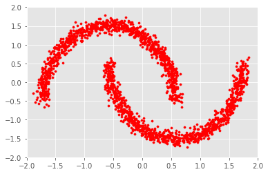
Assume our “in-the-wild” distribution is the very famous “Two Moons” distribution, accessible using the datasets.make_moons function in the package sklearn. If we sample some points from this distribution in 2D-space with 0.05 gaussian noise, it looks like this:

With these techniques, we can take every data point in our data $\{x_j\}_{j=1}^{N}$, and using our change of variables formula, compute the likelihood of the data under the distribution of $Z_T$. We can then optimise the weights of the $f_i$’s so that the likelihood is maximal given the data. As was described above, the $f_i$’s have to take a very specific form, which in this case are picked as RealNVP, which stands for “Real Non Volume Preserving”.

What we end up with is a set of transformations $f^*_{1}, \dots, f^*_{T}$ such that $p(X)$, the likelihood of the data under this model, as was defined above, is maximised. Essentially, we have learned an invertible mapping from $N(0, I)$ to whatever distribution $X$ follows, and we can now sample from this distribution. We can even get an approximation for the probability density function of this distribution.

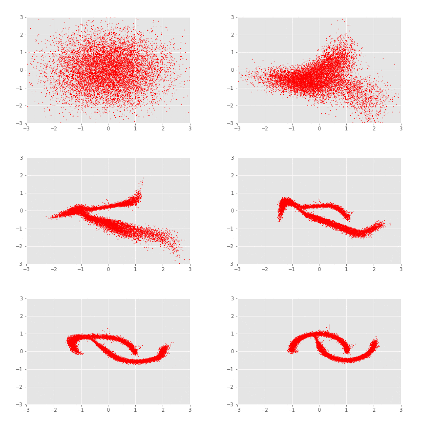
Now there are cool things that we can do. Firstly, we can sample from $Z_0$, then apply the sequence of transformations, allowing us to virtually sample from $Z_T = X$ (as per our model). Another way to validate that your model is working properly, beyond the maximisation of the likelihood, is to apply the sequence of transformations from $f^*_1$ to $f^*_T$ to samples drawn from the $N(0, I)$ distribution and observe whether we recover the “in-the-wild” distribution (i.e. the $x_j$’s). In this case, $T=6$.

And there you have it. These look like a continuous transformation of samples from $N(0, I)$ to samples from $p_{Z_T}(Z_T)$. You can, however, clearly tell that these are just $T$ different discrete transformations, with interpolation in between to make it into a nice GIF. It’s interesting, isn’t it, how it almost seems like these transformations look like rotations.

Now why should we care about the fact that these transformations are actually just discrete, and not continuous? What I mean by this is that if we sample $z_0$, then we can have access to

$z_1 = f_1^*(z_0), z_2 = f_2^*(z_1), \dots, z_T = f^*_T(z_{T-1})$

However, we don’t have access to intermediate representations, eg $z_{1.5}$. In fact, this notation is undefined as of now. What would $z_{1.5}$ even be? We’ll see what this means in part 2 of this tutorial.